Back-to-Back Games — How NBA Fatigue Distorts Prop Lines on Both Nights
 Available in US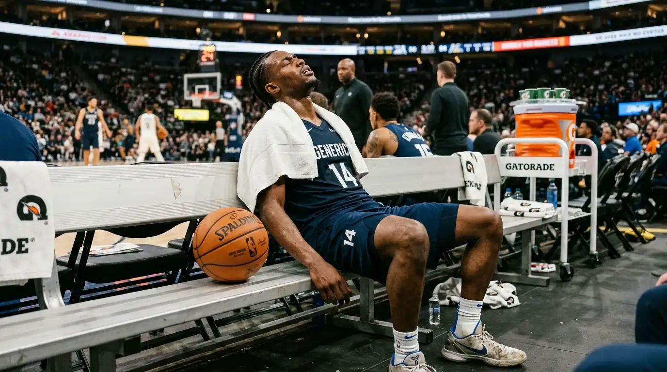
The second night of a back-to-back is the single most distorting condition on the NBA prop calendar, and it shapes both nights of the pair rather than just the second. Punters who think they only need to worry about the second night miss half the picture. The first night of a back-to-back changes player behaviour preemptively — coaches manage minutes, stars conserve effort late, and the game flow shifts because both teams know what is coming the next evening. The prop pricing on both nights reflects this, and the punters who model the back-to-back framework correctly capture small but consistent edges that casual punting leaves on the table.
The data that defines back-to-back fatigue
The shooting numbers on second nights of back-to-backs drop measurably compared to rested nights. League-average effective field goal percentage falls by roughly 1.5 to 2 percentage points on the second night, three-point accuracy falls by a similar amount, and the foul rate rises slightly because tired defenders close out late and contact picks up. Pace is essentially unchanged at the team level — both teams are tired, so the relative tempo holds — but individual minute distributions shift sharply. Stars are more likely to sit, more likely to play restricted minutes when they do play, and more likely to be pulled in the fourth quarter even in close games.
This produces a specific prop pricing pattern. Stars’ lines on second nights are systematically lower than their season averages because operators have priced the fatigue effect carefully. The challenge for punters is that the operator’s adjustment is sometimes too aggressive and sometimes not aggressive enough, depending on the specific player and the specific schedule context. A star who is rested by the team most second nights gets his lines deeply discounted, even when he plays — operators expect him not to play and price accordingly. A star who plays through second nights consistently has his lines discounted but to a smaller degree, and the residual edge sometimes goes to overs.
The under bias on second nights is the punter’s first instinct, and the operator has priced that instinct into the line. Generic second-night unders without specific matchup or player context are not value bets. They are the obvious play that the operator’s model has fully absorbed. The genuine edges are in the specific cases where the operator’s average adjustment over- or under-corrects relative to the player’s actual second-night profile.
The road back-to-back versus the home back-to-back
Travel distance shapes back-to-back impact more than the schedule notation suggests. A team flying coast-to-coast between game one and game two of a back-to-back faces qualitatively different fatigue conditions than a team playing two consecutive home games or two close-distance road games. The cross-time-zone red-eye flight on the night between two games produces measurable drops in shooting accuracy and rebounding effort that travel-controlled studies have documented over decades.
The operator’s pricing model captures travel distance as an input, but the modelling is coarse — most operators treat back-to-backs uniformly with a small modifier for cross-country travel. The reality is more granular. A team flying from the East Coast to the West Coast loses roughly three hours of effective rest because of time-zone shift compounding the late-arrival effect. A team flying west to east on a back-to-back gains time but loses sleep. The directional asymmetry produces specific patterns that show up in scoring data over multi-season samples but that operator pricing models do not always discriminate between.
The most specific edge I have caught in this space is the cross-country red-eye on the second night of a back-to-back where the visiting team’s primary scorer has historically struggled in this specific schedule context. The operator’s average second-night adjustment does not differentiate between the player’s home back-to-back performance (where his averages are minimally affected) and his cross-country back-to-back performance (where his averages drop materially). The under at the headline line carries genuine value in those specific matchups, and the volume across a season is enough to be meaningful.
Coaches’ minute management — the visible fatigue lever
Coaches manage minute exposure across back-to-backs in ways that are visible to anyone watching pre-game press conferences and rotation patterns. A starter who logged 36 minutes the night before will routinely be capped at 28 to 30 minutes on the second night even if the game stays close. A bench player whose role expanded the night before to cover for a rested teammate sometimes returns to his normal smaller role on the second night, even if the original starter sits again. The patterns are coach-specific and roster-specific, and tracking them across the season produces actionable minute projections that beat the operator’s average adjustment.
The way I track this is by maintaining a rolling table of each starter’s minutes across each back-to-back configuration the team has played that season. A starter who has averaged 30 minutes on second nights against the operator’s typical 28-minute projection is a candidate for over bets when the operator’s pricing assumes the lower minute total. Conversely, a starter who has averaged 24 minutes against the same 28-minute baseline is a candidate for unders when the line has not adjusted to his specific pattern.
This kind of granular tracking takes work, but the work compounds across the season. The 250,000 unique prop markets posted across the NBA season include thousands of back-to-back lines, and the consistent edges in this space are not in the headline second-night unders. They are in the player-specific patterns that the operator’s average adjustment misses. Usage rate analysis overlays well with this minute tracking — a player whose usage rate climbs on second nights to compensate for missing teammates is a different prop animal than a player whose usage falls because the team coasts.
The first night that nobody talks about
The front end of a back-to-back changes player behaviour because the players know the second night is coming. Stars often play their normal minutes but conserve effort in stretches where the team has a comfortable lead, knowing they need to be available the next night. The result is a small but measurable drop in fourth-quarter scoring on first nights compared to standalone games for stars on heavy back-to-back schedules.
This effect is subtle and operators have priced it incompletely. The lines on first nights of back-to-backs are typically set as if the games were standalone, with no specific adjustment for the upcoming second night. The error is small — perhaps half a point on a star’s headline scoring line — but it shows up consistently on stars who are also the team’s primary fourth-quarter scorer. The under on these specific lines carries a slim but real edge.
The flip side is that bench players who expect to play heavier minutes on the second night sometimes have their first-night minutes slightly reduced as the coach manages overall workload. The minutes pattern across the back-to-back is more complex than the headline notation suggests, and the punters who model both nights together find pricing inefficiencies that one-night-at-a-time analysis misses.
The three-in-four and four-in-five extreme schedules
Three games in four nights and four games in five nights are the extreme conditions where fatigue effects become genuinely large. Star availability on the third or fourth game of these stretches drops sharply — sometimes by 30 to 40 per cent — and the prop markets respond accordingly. The lines on stars in these conditions are deeply discounted, sometimes more deeply than the actual rest-of-season average performance justifies.
Where the edge appears is when a star is signalled as available for the third or fourth game and the operator’s pricing has applied the full standard discount. If the star is going to play, the discount on his lines represents genuine over value because the operator’s model is pricing for the more likely scenario of him sitting. The signal that he will play is usually given by the team during the morning shootaround or in pre-game press conferences, and the props pricing sometimes does not refresh quickly enough to capture this update.
The volume of these spots is low — perhaps ten to fifteen per season for any specific star — and the edges are short-lived once the operator’s pricing refreshes. Punters who position quickly when the signal appears capture the edge; punters who research overnight and bet at lunchtime miss it. This is one of the spaces where being active on the day of the game pays for itself.
Reading the schedule architecture as research
The NBA schedule is built to balance load across teams, but the balance is imperfect and the imbalances produce systematic prop edges. A team finishing a five-game road trip on the second night of a back-to-back faces a fatigue load that is qualitatively different from a team playing the second of two home games. The schedule context — road trip length, travel cumulative kilometres, time since last home game — shapes player performance in ways that compound the back-to-back adjustment.
Operator models capture some of this but not all of it. The specific compound conditions where multiple fatigue factors stack are where the pricing tends to drift furthest from realised performance. A team finishing its sixth game in nine nights on a coast-to-coast road trip back-to-back is a fatigue extreme that the operator’s pricing model handles as an average of its component adjustments rather than as a non-linear compound effect. The reality is non-linear. Fatigue compounds in ways that the linear adjustments do not capture.
The disciplined approach is to build a fatigue index that combines schedule density, travel cumulative load and individual player minute totals over the previous fortnight. The index produces a single number that rates the fatigue exposure for a given player on a given night, and the prop projections adjust off that number rather than off the simple back-to-back binary. This kind of work is unfashionable because it is unglamorous, but it is the layer of research that produces the consistent edges in this market over multi-season samples. The punters who do it find what they are looking for. The punters who do not, do not.
Are second-night back-to-back unders generally good value bets?
Generic second-night unders without specific matchup or player context are not value bets. Operators have priced the average fatigue effect carefully into second-night lines. The genuine edges are in the player-specific cases where the operator’s average adjustment over- or under-corrects relative to the player’s actual second-night profile, which requires tracking individual back-to-back patterns across the season.
How do coast-to-coast travel back-to-backs differ from short-distance ones?
Cross-country travel on the night between two games produces measurable drops in shooting accuracy and rebounding effort that travel-controlled studies have documented. The operator’s average back-to-back adjustment does not always discriminate between travel-heavy and travel-light back-to-backs, and the cross-country compound effect produces specific under-pricing edges that disciplined punters can capture.
What signals indicate a star will actually play on a fourth-in-five night?
The team usually signals availability during the morning shootaround or in pre-game press conferences. Operator props pricing sometimes does not refresh quickly enough to capture this update, leaving the line at the heavy-discount level priced for the more likely scenario of the star sitting. Quick positioning when the signal appears captures the edge before the line moves.
Published by the nba Best Player Prop Bets team.